Getting started with Josiann
In this tutorial, we introduce the basics of working with Josiann on a simple cost function with noise.
We will show how to define and parametrize cost functions, use multiple move functions and choose parameters of the Simulated Annealing (SA) algorithm.
[1]:
import plotly.io as pio
pio.renderers.default = "png"
[2]:
import numpy as np
import plotly.graph_objects as go

import numpy.typing as npt

import josiann as jo
/home/mbouvier/git/josiann/josiann/algorithms/sequential/base/sa.py:9: TqdmExperimentalWarning:

Using `tqdm.autonotebook.tqdm` in notebook mode. Use `tqdm.tqdm` instead to force console mode (e.g. in jupyter console)
Basic usage
The simplest way to use Josiann is the basic josiann.sa() algorithm. It expects a cost function whose input is a position vector in n dimensions (a numpy.array with shape (n,)), evaluates a function at that position and returns a single float value (i.e. the cost).
Here we will define a function which will square the position vector and add a random noise:
[3]:
def cost_function(x: npt.NDArray[np.float64]) -> float:
    return np.sum(x ** 2) + np.random.normal(0, 3)
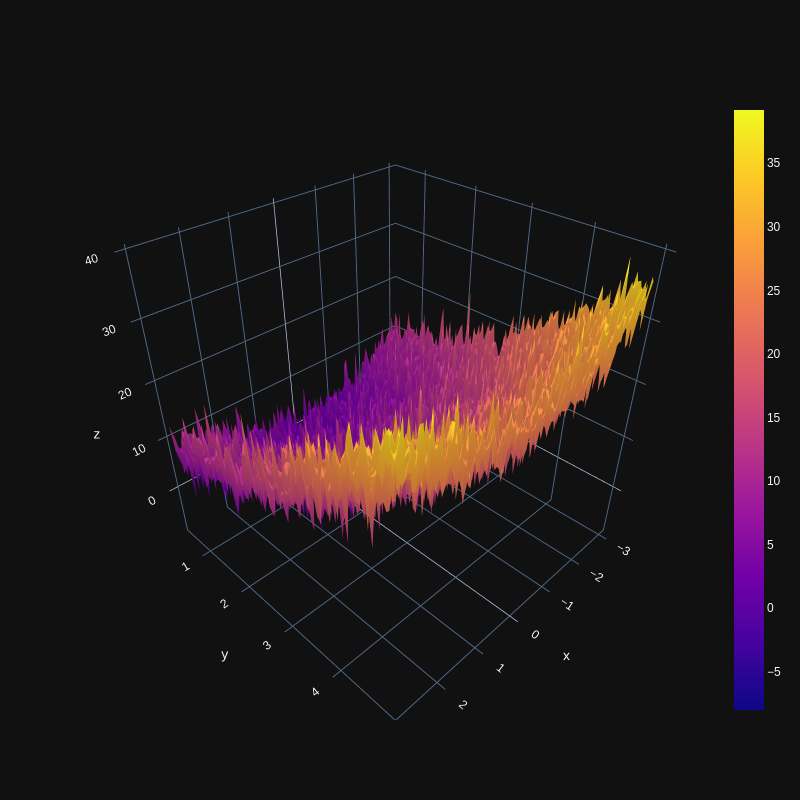
Let’s represent that function when the position vector is in 2D space, bounded by [-3, -3] on the first axis and [0.5, 5] on the second axis. Since we compute the function only once at each position, it has a jagged appearance because of the noise term.
In the absence of noise, the global minimum within the bounds would be easy to find: (0, 0.5).
[4]:
nx, ny = 100, 100

X = np.linspace(-3, 3, nx)
Y = np.linspace(0.5, 5, ny)

xv, yv = np.meshgrid(X, Y)
coords = np.concatenate((xv.flatten()[:, None], yv.flatten()[:, None]), axis=1)
[5]:
fig = go.Figure(data=[go.Surface(x=X, y=Y, z=np.array([cost_function(c) for c in coords]).reshape(nx, ny))])
fig.update_layout(height=800, width=800)
fig.show()
Let’s run Josiann on that function:
We’ll need to pass the cost function as first parameter. The second parameter defines the initial position vector and can be anything within the bounds of the problem (here we pick a position at random).
We then set the bounds of the problem and choose a move function to generate new position vectors. A common move function is the Metropolis move where a new position is drawn at random from a multivariate normal distribution centered on the current position.
Finally, we set parameters of the SA algorithm:
max_iter: the maximum number of iteration to run
max_measures: the maximum number of function evaluations at a given position
T_0: the initial value for the Temperature parameter$
seed: the seed for the random number generator
[6]:
x0 = np.array([[np.random.randint(-3, 4), np.random.choice(np.linspace(0.5, 5, 10))]])

res = jo.sa(cost_function,
            x0,
            bounds=[(-3, 3), (0.5, 5)],
            moves=jo.Metropolis(variances=np.array([0.1, 0.1])),
            max_iter=200,
            max_measures=1000,
            T_0=5,
            seed=42)
[7]:
res
[7]:
Result(
        message: Convergence tolerance reached.
        success: True
        trace: Trace of 187 iteration(s), 1 walker(s) and 2 dimension(s).
        best: [-0.10172863  0.5       ])
Here, we only ran for 187 iterations before Josiann detected it had converged on a solution. The best found position vector was (-0.0771, 0.5), which is really close to the true minimum (0, 0.5).
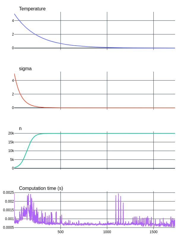
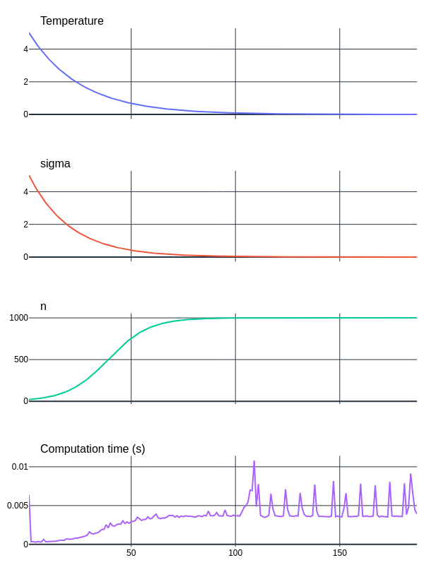
We can obtain details on a run by plotting the evolution of parameters of the SA algorithm.
[8]:
res.trace.plot_parameters()
[9]:
res.trace.plot_positions(true_values=[0, 0.5])

This plot is the most useful of the two: it shows how the position vector changed as iterations were computed, alongside with its associated cost and number of function evaluations (n).
Parametrizing the cost function
Sometimes, we want to use a cost function which accepts more than one input parameter. Josiann can pass additional constant parameters using its args parameter.
As an example, let’s modify the previous cost function by adding a variance parameter to choose the noise level.
[10]:
def cost_function_with_arg(x: npt.NDArray[np.float64], var: float) -> float:
    return np.sum(x ** 2) + np.random.normal(0, var)
We can then run josiann.sa() as previously, passing the variance parameter in args:
[11]:
x0 = np.array([[np.random.randint(-3, 4), np.random.choice(np.linspace(0.5, 5, 10))]])

res = jo.sa(cost_function_with_arg,
            x0,
            args=(3,),                                              # <-- a tuple of positional arguments to pass to
                                                                    # cost_function_with_arg() after the position vector.
            bounds=[(-3, 3), (0.5, 5)],
            moves=jo.Metropolis(variances=np.array([0.1, 0.1])),
            max_iter=200,
            max_measures=1000,
            T_0=5,
            seed=42)
[12]:
res
[12]:
Result(
        message: Convergence tolerance reached.
        success: True
        trace: Trace of 187 iteration(s), 1 walker(s) and 2 dimension(s).
        best: [-0.07414436  0.5       ])
Vectorized cost function
In this example, we will show how to we can speed up Josiann by using vectorized cost functions, discrete moves and a backup system for caching past evaluations.
First, we need to define a vectorized cost function: it should accept a matrix of shape (w, n), where w is the number of nD position vectors for which a cost must be computed, and should return a list of costs of length w.
[13]:
def vectorized_cost_function(x: npt.NDArray[np.float64]) -> list[float]:
    return np.sum(x ** 2, axis=1) + np.random.normal(0, 1, size=len(x))
Then we define how many walkers we want (i.e. in this case: how many function evaluations can be computed at once). This will allow to evaluate the cost function multiple times at the same position vector or at multiple positions quicker.
[14]:
nb_walkers = 10
Finally, we will call the vectorized version of the SA algorithm josiann.vsa() and use a josiann.SetStep as move function.
Because josiann.SetStep is a discrete step (working on a finite set of allow positions), the probability of obtaining the same position vector twice is high and caching past function evaluations becomes interesting. Caching can be enabled by setting the backup argument to true. Compare how long it took to evaluate the cost function in the first run (no caching) vs the second run (caching enabled) here below:
[15]:
x0 = np.array([[np.random.randint(-3, 4), np.random.choice(np.linspace(0.5, 5, 10))] for _ in range(nb_walkers)])

res = jo.vsa(vectorized_cost_function,
             x0,
             bounds=[(-3, 3), (0.5, 5)],
             moves=jo.SetStep(position_set=[np.linspace(-3, 3, 25),
                                            np.linspace(0.5, 5, 19)]),
             nb_walkers=nb_walkers,
             max_iter=2000,
             max_measures=20_000,
             T_0=5,
             seed=42)
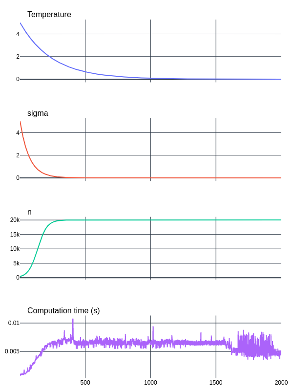
[16]:
res.trace.plot_parameters()
[17]:
res_backup = jo.vsa(vectorized_cost_function,
                    x0,
                    bounds=[(-3, 3), (0.5, 5)],
                    moves=jo.SetStep(position_set=[np.linspace(-3, 3, 25),
                                                   np.linspace(0.5, 5, 19)]),
                    nb_walkers=nb_walkers,
                    max_iter=2000,
                    max_measures=20_000,
                    T_0=5,
                    backup=True,
                    seed=42)
[18]:
res_backup.trace.plot_parameters()